The What

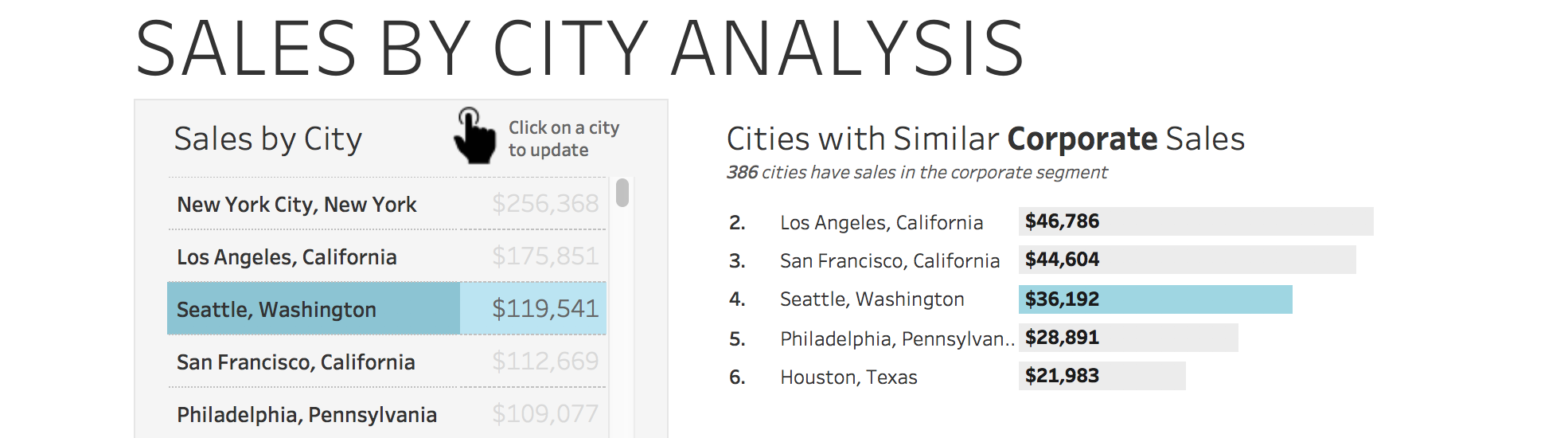
Set actions (along with table calculations) can be used to show dimension values that are similarly ranked to a selected dimension value. For example, selecting the city of Houston will show which 4 cities had sales, in the corporate segment, that were similar to Houston’s corporate segment sales. In this example, “similar” is defined as the two cities that rank above the selected city and the two cities that rank below it. If a city does not have two cities who rank above it, then the four cities ranked directly below it will be shown. The example below could be helpful for managers of a specific city. Say, they wanted to talk to other managers who were experiencing similar sales in a specific category, this would help them find who best to talk to. Or, if a marketing manager wants to run a test in a few different cities, this could allow them to find which cities to include (and which cities could be used as a control).

The Inspiration

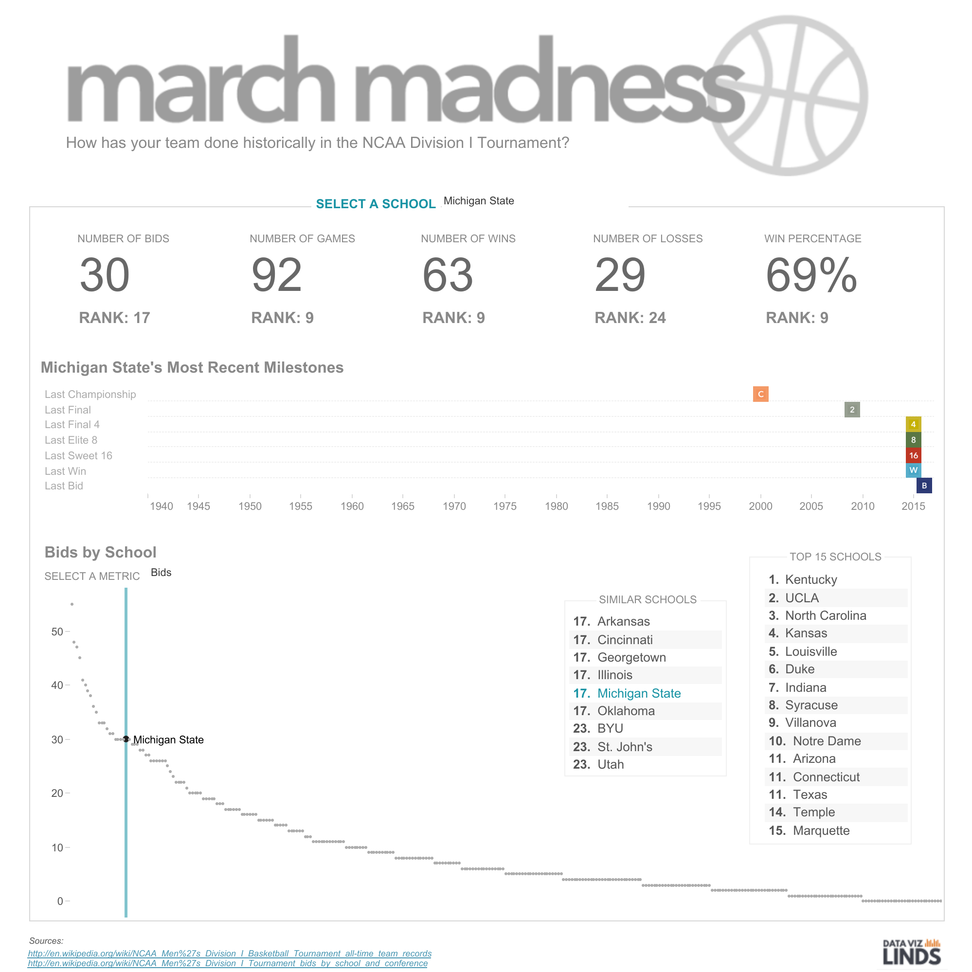
In 2016, I made the following March Madness dashboard. The user selected a school through a parameter and then viewed various information about that school’s success in the NCAA tournament. One of the features of this dashboard was that after you selected a school, you would be able to see 8 schools (four above, four below) with similar stats. I wanted to recreate something similar, except instead of choosing from a parameter dropdown, the user can choose from a table/visualization.

The How

Determine what dimension to use. I am going to choose city to allow me to see which cities rank directly above and below the selected city for any dimension/metric I choose.
Create a new worksheet called “Cities List”. Then, create a new calculation called location. I want the user to see the city and the state, so I am going to create a new calculation to allow me to have a dimension that is formatted as “City, State”.
```
[City] + ", " + [State]
```
Add location to the rows shelf (be careful not to add the hierarchy item called location, but instead the calculation created previously). Add a desired metric, such as sales, to the columns shelf. Sort descending by the field name of sales with an aggregation of sum. This worksheet will serve as what the user interacts with to select a city.
Create a new set based off of the selected dimension, location. To do this, right click on location in the dimension shelf and select create > set. Name the set “Location Set”. Select a value of “San Francisco, California” in order to allow us to have something in the set until we set up the set action.
Create a new calculation called “Similar in Rank”. This will then be able to be used as a filter to only show items that are ranked above and below. In this calculation we will define how many items above and below to include. For this example, I am going to choose to show the two cities ranked above, the two cities ranked below, and the selected city.
```
LOOKUP(ATTR([Location Set]),1)
OR 
LOOKUP(ATTR([Location Set]),2)
OR 
LOOKUP(ATTR([Location Set]),0)
OR
LOOKUP(ATTR([Location Set]),-1)
OR 
LOOKUP(ATTR([Location Set]),-2)
```
What is this calculation actually doing?!
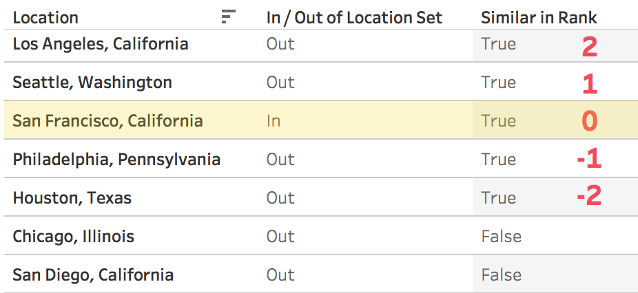
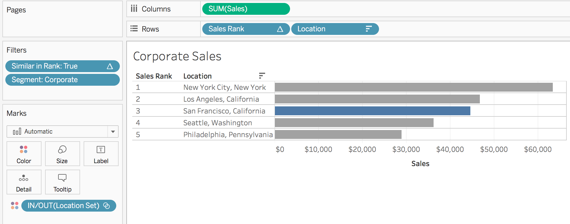
Adding location set to a calculation will return a value of True (In) or False (Out). As demonstrated below, San Fran is selected in the location set, so it returns a value of in, while every other city is out. Lookup() returns the value in the specified number of rows above or below. On the Seattle row for example, LOOKUP(ATTR([Location Set]),1) returns true because the location set value for 1 row below it is true. However, on the Seattle row LOOKUP(ATTR([Location Set]),2) returns false, because it is returning the location set value for Philadelphia. The calculation when applied returns a value of true or false. This is because using the OR to separate the arguments is saying for the current row does 1 or 2 rows above it or 1 or 2 rows below it or the row itself have a location set value of in/true? If any of the specified rows do, return true, else false.

A note with using lookup(): we did not specify a metric anywhere. The calculation is performed purely by what is above and below a row in the table, so how the table/graph is sorted is extremely important to ensure this works!

If you desire to show 3 rows above and 3 rows below, simply add on to the calculation by copying one of the existing arguments and swapping out the number on the end.
Create a new worksheet called “Corporate Sales”. Here we are going to show which cities rank similarly to the selected city in terms of sales in the corporate segment.
Add location to the rows shelf and sales to the columns shelf. Sort descending by the field name of sales with an aggregation of sum. Change the mark to bar.
Add location set to the colors shelf for a quick way to identify the selected city
Create a new calculation called sales rank. This step is optional, but will allow for a quick indication of how the selected city ranks overall and be a clear indication that the shown cities are ranked above and below.
```
RANK(SUM([Sales]))
```
Add sales rank to the rows shelf, change to discrete, and then move the pill in front of location.
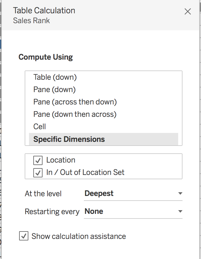
Click on the blue sales rank pill on the rows shelf and select edit table calculation. Select compute using specific dimensions and check the in/out of location set option (while also keeping location checked).
Your view should now look like this
Add similar in rank to the filters shelf and select true
Click on the similar in rank pill on the filters shelf and select edit table calculation. Same as in step 11, change the compute using to specific dimensions and check the in/out location set box (while also keeping location checked).
Click on the similar in rank pill on the filter shelf again and select edit filter. Because we changed the scope of the calculation, it ignored that we had previously selected true. Update the filter once again to only show true.
Add segment to the filters shelf and select corporate. Your view should now look like this:
Create a new dashboard and add the cities list and corporate sales worksheets
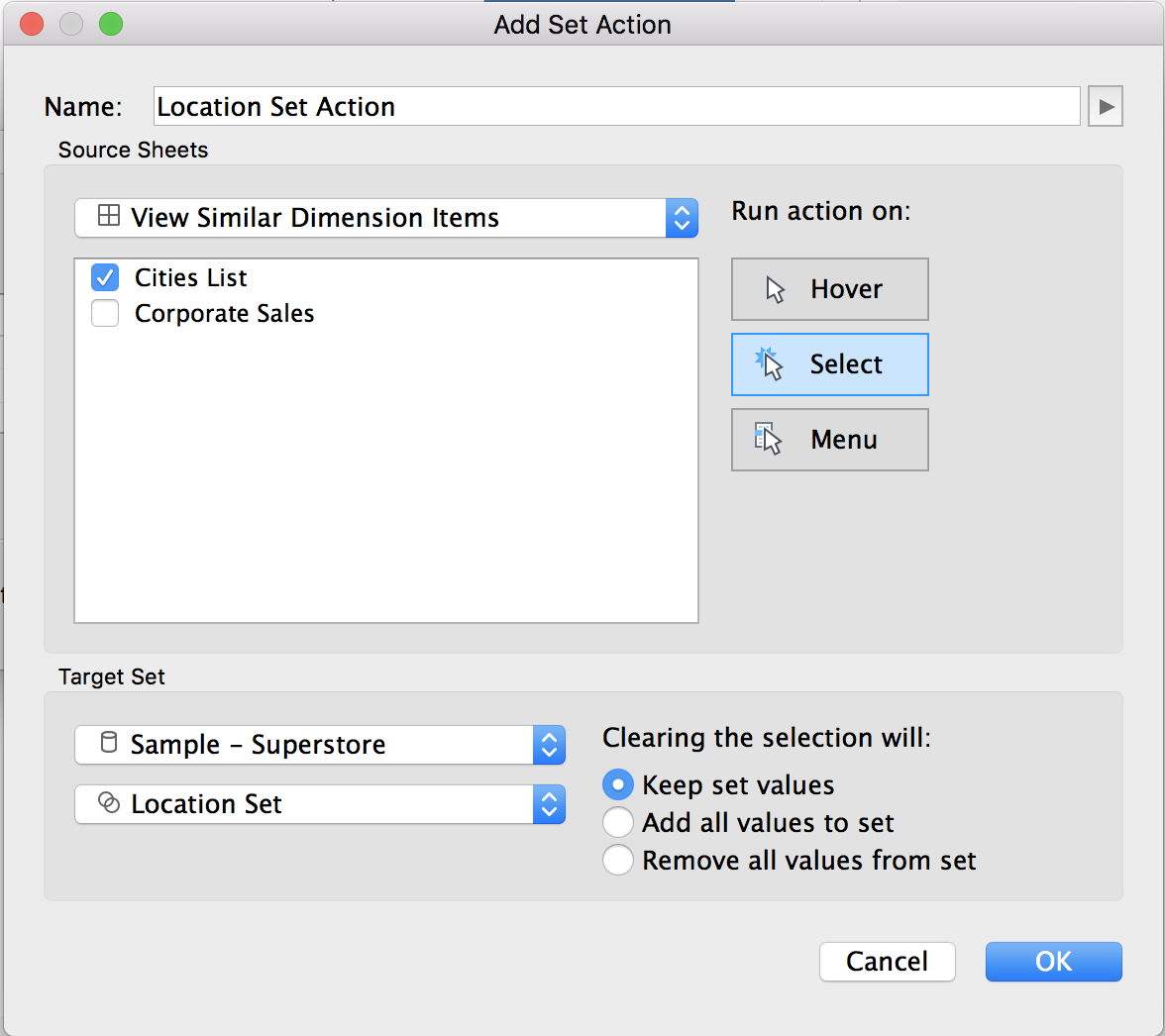
On the dashboard, add a new set action. This can be done by going to worksheet > actions > add action > change set values. Run the action on select, with clearing the selection will keep set values. Only run the action on the cities list worksheet.
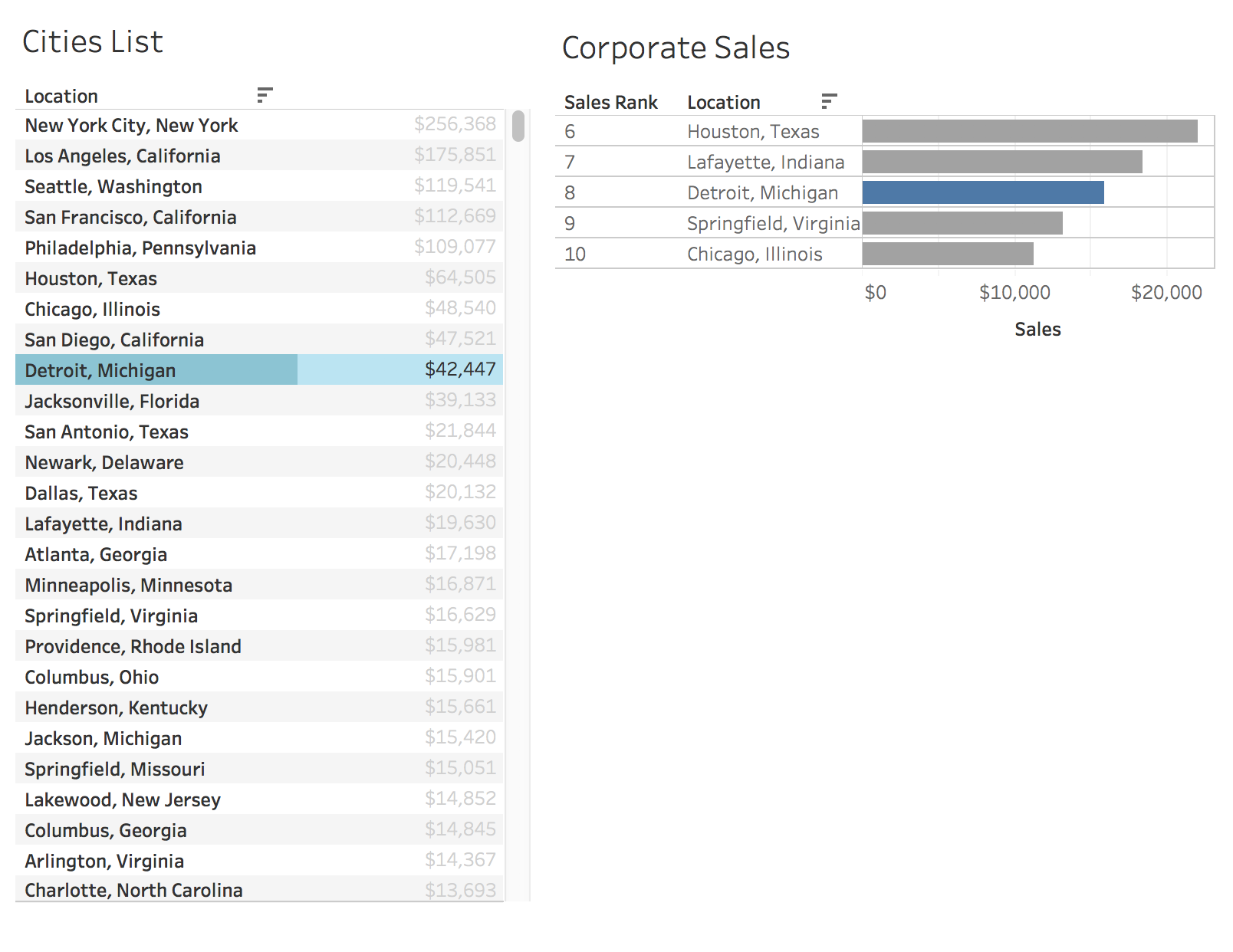
Test it out! Click on a location and watch the bar graph update. Springfield, Virginia ranks directly below Detroit in corporate sales…. but ranks 8 below Detroit in overall sales!
The corporate sales worksheet can now be duplicated and any filters can be applied/swapped out and the worksheet is good to go (say if you wanted to look at technology sales). The measure can also be changed if you wanted to look at cities with similar profit (just don’t forget to duplicate the sales rank calculation and swap in profit AND to sort cities by profit to ensure the lookup works correctly)
Duplicate the corporate sales worksheet and call it technology sales. Remove the corporate segment filter and add category to the filters shelf. Select a category of technology.
Duplicate the corporate sales worksheet again and call it state sales. Remove the corporate segment filter. This time, we are going to look at the rankings within the state of the selected city. So, for example, when Los Angeles is selected, we will be able to see the other California cities that are ranked above/below it.
Create a new calculation called selected state. This calculation is saying if a value is in the location set, then return the state. However, we need to wrap it in a LOD to allow us to apply that value to every row in the data set. Then, by setting that equal to state, it will only return values where the two states are the same.

{MIN(if [Location Set] then [State] END)}=[State]

Add selected state to the filters shelf and select true.
Add the technology sales and selected state worksheet to the dashboard and test it out again!
Additional tips:
- A city such as New York is ranked at the very top and therefore does not have two cities ranked above it. Instead of leaving it to only show 3 cities (New York City + two cities below), update the similar in rank calculation to show 4 cities below… so there are always 5 total cities showing! Add this to the bottom of the similar in rank calculation
- ```
OR 
LOOKUP(ATTR([Location Set]), IF ISNULL(LOOKUP(ATTR([Location Set]),-4)) then -3 end)OR 
LOOKUP(ATTR([Location Set]), IF ISNULL(LOOKUP(ATTR([Location Set]),-5)) then -3 end)OR 
LOOKUP(ATTR([Location Set]), IF ISNULL(LOOKUP(ATTR([Location Set]),-5)) then -4 end)OR
LOOKUP(ATTR([Location Set]), IF ISNULL(LOOKUP(ATTR([Location Set]),4)) then 3 end) 
OR 
LOOKUP(ATTR([Location Set]), IF ISNULL(LOOKUP(ATTR([Location Set]),5)) then 3 end)
OR 
LOOKUP(ATTR([Location Set]), IF ISNULL(LOOKUP(ATTR([Location Set]),5)) then 4 end)
```
- Bar Chart Formatting:
  - Unshow the header/axis
  - Change the fit to entire view
  - Remove row and column dividers
  - Remove column gridlines
- Format the “Sales Rank” calculation using custom number formatting. Update it to #,##0. (this adds a period at the end of the rank to make it look more like a list). Resize the column to make the sales rank smaller
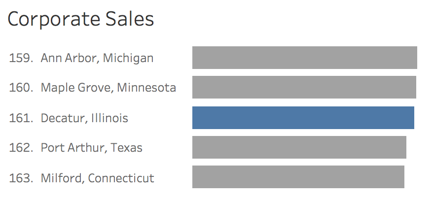
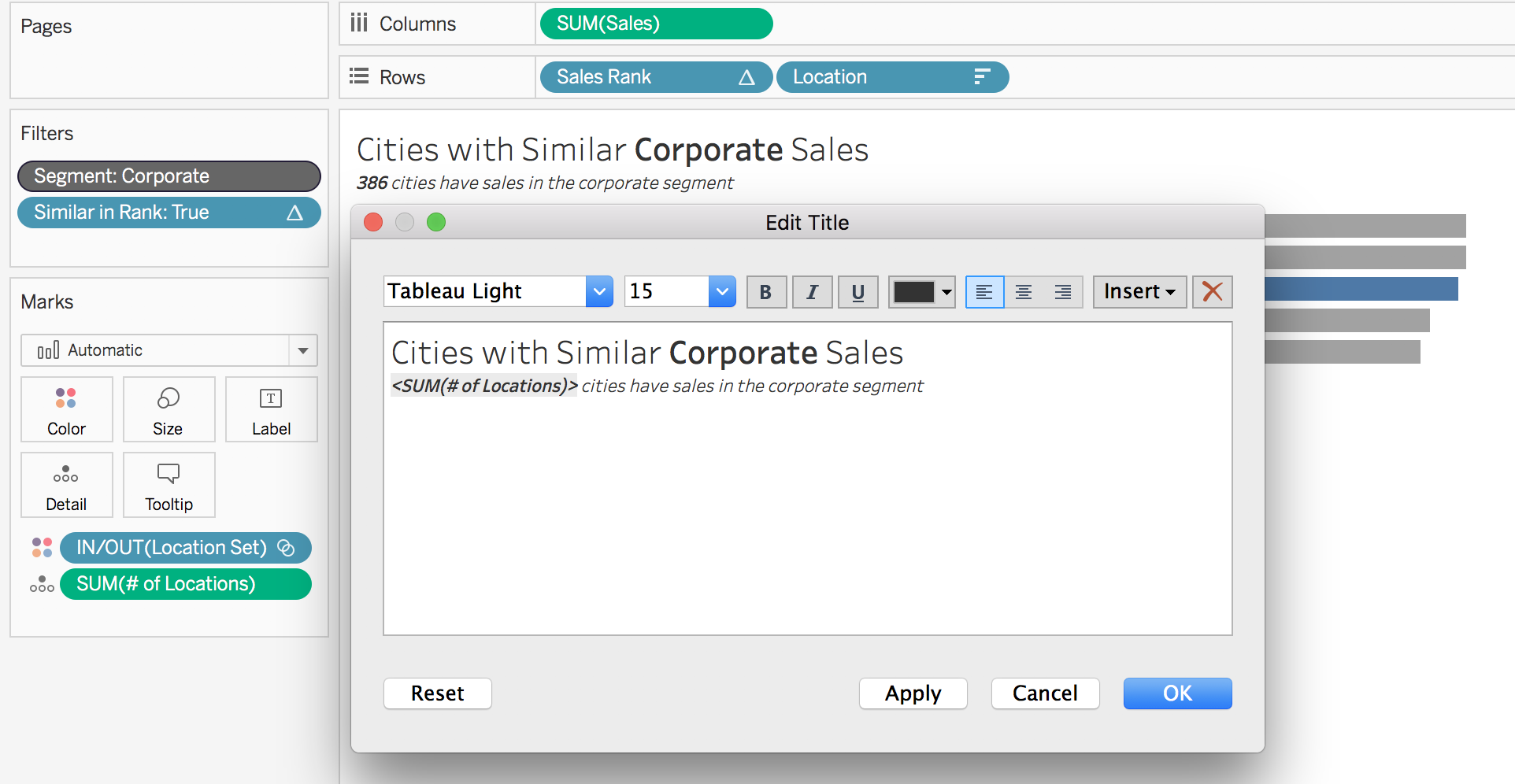
- Underneath the title of the worksheet, add context about how many cities are available to be ranked. For example, there are 604 cities in the dataset, but only 386 have sales in the corporate segment. In the image above, it would be helpful to know if Decatur is ranked 161, what that is out of. To do this, create a new calculation called # of locations
```
{fixed: COUNTD([Location])}
```
  Add it the detail mark and then edit the title to reflect desired wording. Then, whatever filters are on the worksheet (minus the similar in rank one), add to context

To view my working example on Tableau Public or to download my workbook, click here. Also, check out the other dashboards in the workbook detailing different ways to use set actions.